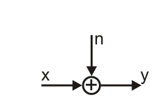
The Additive White Gaussian Noise (AWGN) channel is one of the most important channel models in communications. In this webdemo, we explore its underlying probability distribution, the normal (Gaussian) distributions. The channel model is given by $$ y = x + n $$ where $n$ is Gaussian distributed, with the probability density function (PDF) $$ p_n (\xi) = \frac{1}{\sqrt{2\pi}\sigma}\cdot e^{-\frac{1}{2\sigma^2}\cdot \xi^2}. $$ with $$ \int_{-\infty}^{\infty}{p_n(\xi) d\xi} = 1. $$ Here, $\sigma$ is called the standard deviation and $\sigma^2$ the variance of $n$. Furthermore, $n$ has mean 0.

For a real-valued channel, we define the Signal-to-Noise-ratio (SNR) as $$ SNR_s = \frac{P_s}{P_n} = \frac{E_s}{\sigma^2} \qquad \text{and} \qquad SNR_s\vert_\mathrm{dB} = 10 \log_{10} \frac{E_s}{\sigma^2} $$ where we usually normalize the signal power to $E_s = 1$.

For a complex-valued channel, both the real and the imaginary part experience a Gaussian noise of variance $\sigma^2$, and therefore we have $P_n=2\sigma^2$. As the SNR, we have $$ SNR_s = \frac{P_s}{P_n} = \frac{E_s}{2\sigma^2} \qquad \text{and} \qquad SNR_s\vert_\mathrm{dB} = 10 \log_{10} \frac{E_s}{2\sigma^2}. $$