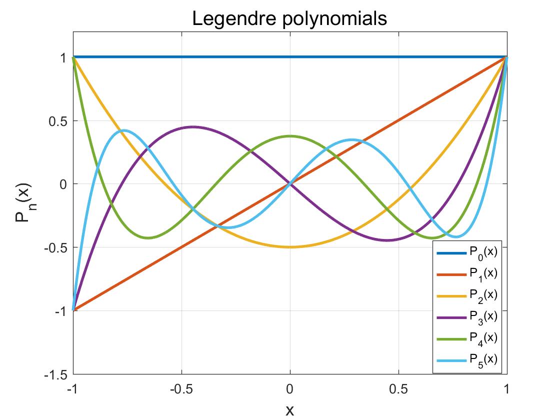
The Legendre polynomials are selected as the basis functions, which are used to estimate the channel transfer function. The channel transfer function $\mathbf{H}_{n}$ within a short time period (i.e., determined by sliding window length) at the $n$-th subcarrier can be modeled as a linearly weighted sum of some basis functions.

$$\mathbf{H}_{n}=\mathbf{G}\cdot\boldsymbol{\theta}+\mathbf{Z}=\sum_{i=0}^{V}\Phi_{i}\left(n\right)\cdot\theta_{i}+\mathbf{Z}$$

where
$\mathbf{G}$ denotes the polynomial matrix evaluated within the sliding window duration,
$\Phi_{i}\left(k\right)$ is the $i$-th basis function evaluated at the $k$-th symbol time,
$\theta_{i}$ is the weighting factor of the basis function $\Phi_{i}\left(k\right)$,
$V$ is the highest order of used basis polynomials,
$\mathbf{Z}$ is the noise.

Exploiting the estimated channel at pilot positions $\hat{\mathbf{H}}_{n}$, the weighting factor $\hat{\boldsymbol{\theta}}_{LS,n}$ can be calculated by

$$\hat{\boldsymbol{\theta}}_{LS,n}=\left(\mathbf{G}_{p}^\mathrm{H}\mathbf{G}_{p}\right)^{-1}\mathbf{G}_{p}^\mathrm{H}\cdot\hat{\mathbf{H}}_{n},$$ where $\mathbf{G}_{p}$ denotes the polynomial matrix evaluated at pilot positions.

Then, channel $\hat{\mathbf{H}}_{LS,n}$ at all non-pilot positions $k$ can be estimated by

$$\hat{\mathbf{H}}_{LS,n}=\mathbf{G}\cdot\hat{\boldsymbol{\theta}}_{LS,n}=\sum_{i=0}^{V}\Phi_{i}\left(k\right)\cdot\hat{\theta}_{LS,n}\left(i\right)$$

The interpolation in the frequency domain is the same as that in the time domain.

The figure shows the Legendre polynomials up to the 5th order, which are orthogonal to each other in [-1,1]. Note that the used maximal Legendre polynomial order is half of the sliding window (SW) length.