We extend the LS interpolation to another type polynomials, which are referred to as eigen-functions.

The time correlation of a single-tap channel in rich scattering environments is given by

$$R_{t}\left(t\right)=J_{0}\left(2\pi f_{D}t\right)$$

where $J_{0}\left(\cdot\right)$ is the zero-th order Bessel function of the first kind and $f_{D}$ the maximum Doppler shift.

Consider again the channel transfer function $\mathbf{H}_{n}$ within sliding window time at $n$-th subcarrier, the auto-covariance matrix $\mathbf{R}_\mathrm{d}$ is defined by $$\mathbf{R}_{\mathrm{d}}=\mathrm{E}\left(\mathbf{H}_{n}\cdot\mathbf{H}_{n}^{^{\mathrm{H}}}\right),$$ where $\mathbf{R}_{d}$ is a Toeplitz matrix consisting of $R_{t}\left(t\right)$.

Applying eigenvalue decomposition, $\mathbf{R}_{\mathrm{d}}$ can be written as

$$\underset{N_{S}\times N_{S}}{\underbrace{\mathbf{R}_\mathrm{d}}}=\underset{N_{S}\times D}{\underbrace{\mathbf{Q^{\mathrm{H}}}}}\cdot\underset{D\times D}{\underbrace{\boldsymbol{\Lambda}}}\cdot\underset{D\times N_{S}}{\underbrace{\mathbf{Q}}}$$

where
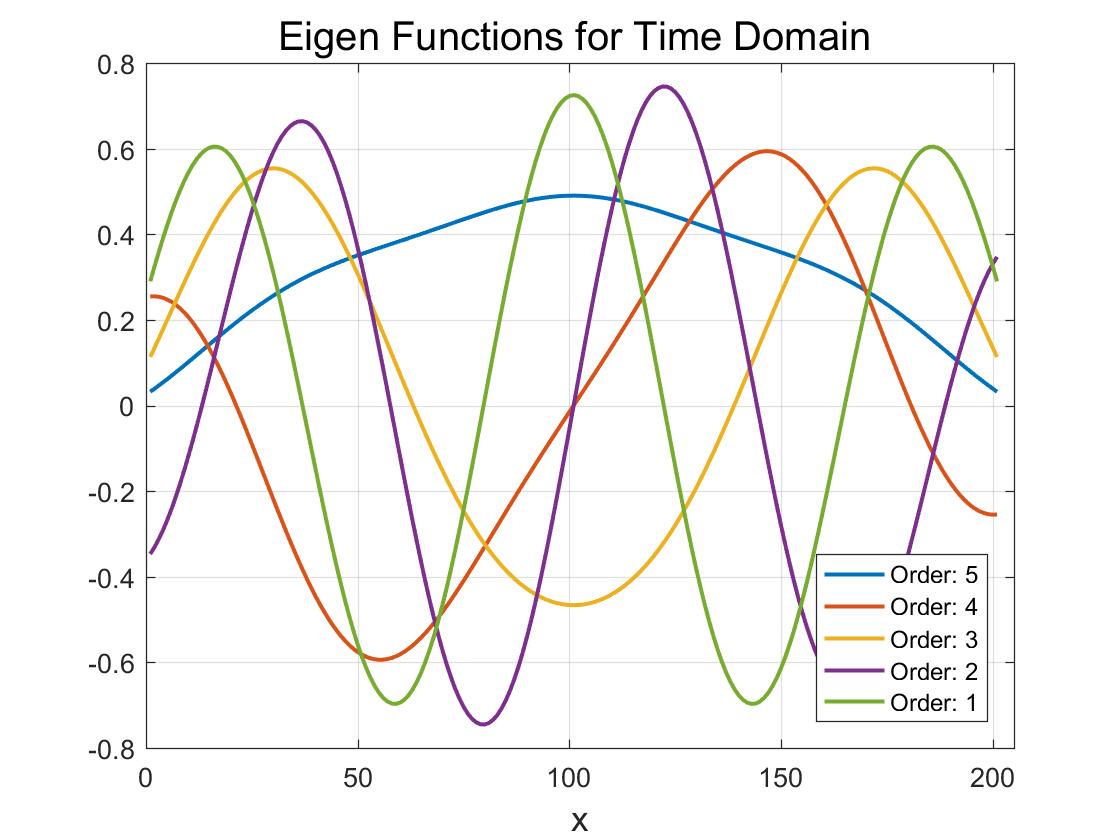
the rows of $Q^{\mathrm{H}}$ constitute perfect polynomials for time domain interpolation,
$D$ is the rank of $Q^{\mathrm{H}}$ and $N_{S}$ is the total number of symbols in the time domain.

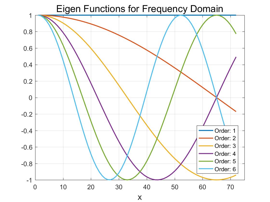
In the frequency domain, we use DFT matrix $\mathbf{F}^{\mathrm{H}}$ as polynomials.

$$\mathbf{R}_{F}=\mathbf{F}^{\mathrm{H}}\cdot\mathbf{P}\cdot\mathbf{F}$$

where $\mathbf{P}$ is the PDP of channel and $\mathbf{R}_{F}$ is the auto-covariance matrix of channel coefficients in the frequency domain.

The calculation of channel estimator is the same as that in LS with Legendre polynomials.

The eigen functions in the time and frequency domain are shown in the figures below, respectively.