Properties
For a quick introduction to LDPC codes, see webdemo LDPC Codes from Communication Standards or Peeling Decoder for Graph Based Codes. The LDPC code defined in the 5G standard is a protograph-based, irregular, systematic and quasi-cyclic code.
• Protograph-based: For the 5G LDPC code two base graphs (or protographs) are defined, each of which provides different permuting matrices $\mathbf{B}$. The codes parity-check matrix $\mathbf{H}$ is constructed from $\mathbf{B}$ by so-called lifting.
• Quasi-cyclic: Cyclically shifting parts of a codeword will result in another valid codeword. The described lifting process results in this property.
• Irregular: A LDPC code is called regular, when each column of $\mathbf{H}$ contains $w_{\mathrm{c}}$ 1’s, each row contains $w_{\mathrm{r}}$ 1’s and $w_{\mathrm{c}}=w_{\mathrm{c}}\cdot\frac{n}{n-k}$, otherwise it is called irregular. Irregularity is typical for capacity approaching LDPC codes.
• Systematic: A code is called systematic, if each codeword $\mathbf{c}$ contains both the input symbols $\mathbf{u}$ and the parity symbols $\mathbf{p}$. Codewords of the 5G LDPC code are structured like this $\mathbf{c}=\begin{pmatrix} u_{1},&u_{2},&\dots,&u_{K},&p_{1},&p_{2},&\dots,&p_{N-K}\end{pmatrix}$.
Structure
The two base graphs, BG1 and BG2, are represented by their respective base matrix $\mathbf{H}'_{\mathrm{BG1}}$ and $\mathbf{H}'_{\mathrm{BG2}}$. Their structure is as follows. $$ \mathbf{H}'=\begin{bmatrix} \mathbf{M'} & & \mathbf{D'} & & \mathbf{0}\\ & \mathbf{E'} & & & \mathbf{I} \end{bmatrix}, $$ where the main part $\mathbf{M'}$ is a high density matrix, $\mathbf{D'}$ is a $4 \times 4$ double-diagonal structured matrix, $\mathbf{0}$ is an all zero matrix, the extension part $\mathbf{E'}$ is a low density matrix and $\mathbf{I}$ is an identity matrix. $\mathbf{H_{\mathrm{BG1}}}'$ has dimensions $46 \times 68$ and $\mathbf{H_{\mathrm{BG2}}}'$ is a $42 \times 52$ matrix. The following figures display both base matrices.
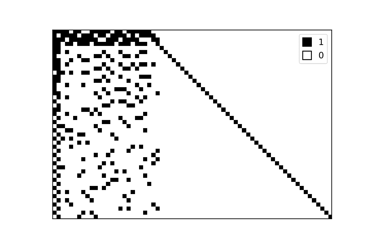
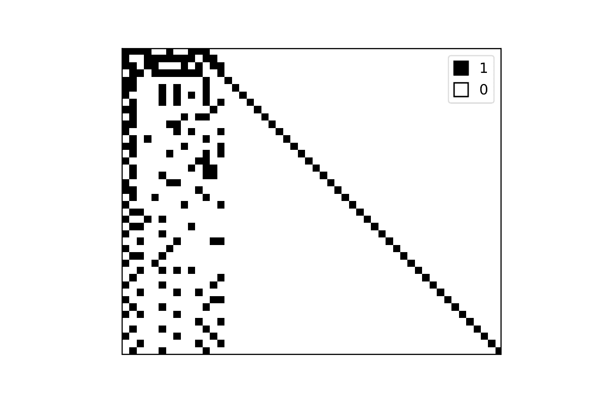
Notice that the first two columns of $\mathbf{H}'_{\mathrm{BG1}}$ and $\mathbf{H}'_{\mathrm{BG2}}$ are comparably dense. This will be considered for the rate matching.
Every parity check matrix has the same structure as the used base graph. In the following $\mathbf{E}$, $\mathbf{M}$ and $\mathbf{D}$ will denote the corresponding parts of $\mathbf{H}$, similar to the notation above.
Code Construction
Depending on the desired parameters, e.g. $K$ and $N$, the following steps are performed to construct the code.- Base graph selection
- Lifting
- Rate-matching
$\mathbf{H}$ is constructed from $\mathbf{B}$ by lifting. Each entry $B_{i,j}$ of $\mathbf{B}$ is replaced by $\mathbf{I}\left(B_{i,j}\right)$, where $\mathbf{I}\left(x\right)$ denotes a matrix of dimension $Z \times Z$, being an identity matrix shifted by $x$ for $x\geq 0$ and all zero for $x=-1$. Lifting allows for the construction of arbitrarily large codes, depending on the lifting size $Z$ and the permuting matrix $\mathbf{B}$. As an example we assume a small base graph defined by $$ \mathbf{H}'_{BG}=\begin{bmatrix} 1 & 0 & 1 & 0 \\ 1 & 1 & 1 & 1 \end{bmatrix}. $$ The permuting matrix has the same structure and simply describes the shift of the identity matrices. This corresponds to the edge permutation of the base graph copies. For lifting size $Z=3$ we assume a permuting matrix $$ \mathbf{B}=\begin{bmatrix} 1 & -1 & 0 & -1 \\ 0 & 1 & 2 & 0 \end{bmatrix}. $$ After lifting this will result in the parity check matrix $$ \mathbf{H}=\begin{bmatrix} 0 & 1 & 0 & 0 & 0 & 0 & 1 & 0 & 0 & 0 & 0 & 0 \\ 0 & 0 & 1 & 0 & 0 & 0 & 0 & 1 & 0 & 0 & 0 & 0 \\ 1 & 0 & 0 & 0 & 0 & 0 & 0 & 0 & 1 & 0 & 0 & 0 \\ 1 & 0 & 0 & 0 & 1 & 0 & 0 & 0 & 1 & 1 & 0 & 0 \\ 0 & 1 & 0 & 0 & 0 & 1 & 1 & 0 & 0 & 0 & 1 & 0 \\ 0 & 0 & 1 & 1 & 0 & 0 & 0 & 1 & 0 & 0 & 0 & 1 \end{bmatrix}. $$ In the 5G standard many different lifting sizes are supported, ranging from $Z=2$ to $Z=384$.
Additional rate matching is subsequently applied to tailor the code to the desired $K$ and $N$. The different rate-matching methods are explained on the next page.
Each step and the selection of related parameters is described precisely in the standard, as there are different $\left(N,K\right)$ LDPC codes that can be constructed from the same base graph.