This webdemo computes the channel capacity of an AWGN channel under various constraints.

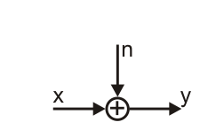
The channel model is depicted in the graph:
Input signal $x$ is affected by $n$ which is additive white Gaussian noise with zero mean and variance $\sigma_n^2$. The receive signal is $y$.
The signals $x$, $n$, and $y$ are real valued. Throughout this webdemo, $n\in\mathbb{R}$ and $y\in\mathbb{R}$ holds, whereas the range of $x$ is limited depending on selected channel type and maximization constraint.

The webdemo computes the channel capacity which is $$C=\max_{X} I(X;Y)$$ with $I(X;Y)$ being the mutual information between $X$ and $Y$. Moreover, the capacity achieving probability density function (pdf) of $X$ is also computed: $$p_X(x) = \arg \max_{X} I(X;Y)$$ The maximization is performed by means of convex optimization. For details, see slide 5 "Theory of Operation", where also the source code can be downloaded.

The user can select between the following channels:

• unipolar channel, i.e. $x\in\mathbb{R}^+$
• bipolar channel, i.e. $x\in\mathbb{R}$

and the following constraints:

• mean power constraint, i.e. $\mathbb{E}\left[x^2 \right] = 1$
• average amplitude constraint, i.e. $\mathbb{E}\left[x \right] = 1$
• amplitude constraint, i.e. $\max |x| = 1$