Transmitted signal
 In the following demo, we compare properties of different waveforms in time and frequency domain from the view of a spectrum analyzer.
To explore the properties of different waveform technologies, we assume that only one subcarrier carries data and only one symbol is transmitted.
The received signal can be written as
$$
s(t)= g(t)e^{j2\pi f_{\rm{sub}}n_{0}t}
$$
where $n_{0}$ denotes an arbitrary subcarrier index, $f_{\rm{sub}} = \frac{1}{T_{s}}$ denotes the subcarrier spacing and $g(t)$ is the pulse shaping filter.
Generally, the transmitted signal has finite duration in time, i.e.
$$
g(t)=0, \quad \textrm{for } \quad |t|>\frac{T_{\textrm{max}}}{2}
$$
where $T_{\textrm{max}}$ is the maximum duration of $g(t)$.
In the following demo, we compare properties of different waveforms in time and frequency domain from the view of a spectrum analyzer.
To explore the properties of different waveform technologies, we assume that only one subcarrier carries data and only one symbol is transmitted.
The received signal can be written as
$$
s(t)= g(t)e^{j2\pi f_{\rm{sub}}n_{0}t}
$$
where $n_{0}$ denotes an arbitrary subcarrier index, $f_{\rm{sub}} = \frac{1}{T_{s}}$ denotes the subcarrier spacing and $g(t)$ is the pulse shaping filter.
Generally, the transmitted signal has finite duration in time, i.e.
$$
g(t)=0, \quad \textrm{for } \quad |t|>\frac{T_{\textrm{max}}}{2}
$$
where $T_{\textrm{max}}$ is the maximum duration of $g(t)$.
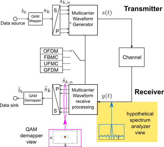
Analysis based on the view of a hypothetical spectrum analyzer
Depending on waveform technique, the length of signal ($T_{\textrm{max}}$) varies, e.g. $T_{\textrm{max}}=8T_{s}$ in FBMC with overlap factor of 4 and $T_{\textrm{max}}=T_{s}$ in OFDM without the insertion of cyclic prefix. The signal is analyzed at receiver by performing FFT after applying windowing $w(t)$ and zero padding. This window is shifted in time and signal is analyzed successively. The spectrum of received signal at time shift $\tau$ is expressed as $$ S(f,\tau) = \mathcal{F}(w(t-\tau)\cdot s(t)) $$ This measure, $S(f,\tau)$, gives a vivid view of energy distribution of arbitrary waveform in time and frequency domain. The length and shape of the adopted window $w(t)$ can be specified. By default, the window is with length of $T_{s}$ and with a rectangular shape in time domain. However, the receiver processing of waveform techniques such as FBMC, UFMC and GFDM is based on signal observation of duration $T_{\textrm{max}}$. To allow signal analysis for arbitrary waveforms, we also provide the possibilities to adapt the window length and shape. The length of window can be specified as $\beta T_{s}$, where $\beta$ can be arbitrary positive value. Available window types are til now
- rectangular, $w(t)=\textrm{rect}(\frac{t}{\beta T_{s}}), t \in [-\beta\frac{T_{s}}{2}, \beta\frac{T_{s}}{2}]$
- Hann, $w(t)=\frac{1}{2}+\frac{1}{2}\cos (\frac{2\pi t}{\beta T_{s}}), t \in [-\beta\frac{T_{s}}{2}, \beta\frac{T_{s}}{2}]$ [9]
- flat-top, $w(t)=1+1.93\cos (\frac{2\pi t}{\beta T_{s}})-1.29\cos (\frac{4\pi t}{\beta T_{s}})+0.388\cos (\frac{6\pi t}{\beta T_{s}})-0.028\cos (\frac{8\pi t}{\beta T_{s}}), t \in [-\beta\frac{T_{s}}{2}, \beta\frac{T_{s}}{2}]$ [9]