Amplified fiber link
 This Webdemo shows how signal power, optical signal-to-noise ratio (OSNR) and
accumulated dispersion evolve along an optical fiber communication link. The
total transmission distance $\ell_\mathrm{tot}$ is divided into $N$ spans of
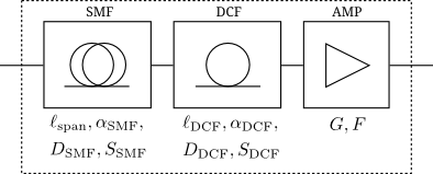
identical length $\ell_\mathrm{span}=\ell_\mathrm{tot}/N$. Each span consists of
a single-mode fiber (SMF), a dispersion compensating fiber (DCF) and an optical
amplifier (AMP) as shown in the figure. The length $\ell_\mathrm{DCF}$ of the
DCF is chosen automatically so that it compensates for the dispersion caused by
the SMF. Similarly, the gain $G$ of the AMP makes up for the loss in optical
power caused by SMF and DCF.
The dispersion coefficient $D_\mathrm{SMF}$ and the dispersion slope
$S_\mathrm{SMF}$ of the SMF are fixed with
$D_\mathrm{SMF}=17\,\mathrm{ps/(nm\cdot km)}$ and
$S_\mathrm{SMF}=0.053\,\mathrm{ps/(nm^2\cdot km)}$. The dispersion coefficent and
slope of the DCF can be chosen freely but its length is calculated
automatically, with
$\ell_\mathrm{DCF}=-\ell_\mathrm{SMF}D_\mathrm{SMF}/D_\mathrm{DCF}$. All
dispersion coefficients and slopes are valid at a wavelength of 1550 nm.
For the power plot only one wavelength is considered (single-channel). The
OSNR refers to a bandwidth of 12.5 GHz.
For the dispersion plot a wavelength division multiplex (WDM) system with 80
channels and center wavelength 1550 nm is assumed. The plot shows the
accumulated dispersion of the channels with lowest, highest and center
wavelength, respectively.
This Webdemo shows how signal power, optical signal-to-noise ratio (OSNR) and
accumulated dispersion evolve along an optical fiber communication link. The
total transmission distance $\ell_\mathrm{tot}$ is divided into $N$ spans of
identical length $\ell_\mathrm{span}=\ell_\mathrm{tot}/N$. Each span consists of
a single-mode fiber (SMF), a dispersion compensating fiber (DCF) and an optical
amplifier (AMP) as shown in the figure. The length $\ell_\mathrm{DCF}$ of the
DCF is chosen automatically so that it compensates for the dispersion caused by
the SMF. Similarly, the gain $G$ of the AMP makes up for the loss in optical
power caused by SMF and DCF.
The dispersion coefficient $D_\mathrm{SMF}$ and the dispersion slope
$S_\mathrm{SMF}$ of the SMF are fixed with
$D_\mathrm{SMF}=17\,\mathrm{ps/(nm\cdot km)}$ and
$S_\mathrm{SMF}=0.053\,\mathrm{ps/(nm^2\cdot km)}$. The dispersion coefficent and
slope of the DCF can be chosen freely but its length is calculated
automatically, with
$\ell_\mathrm{DCF}=-\ell_\mathrm{SMF}D_\mathrm{SMF}/D_\mathrm{DCF}$. All
dispersion coefficients and slopes are valid at a wavelength of 1550 nm.
For the power plot only one wavelength is considered (single-channel). The
OSNR refers to a bandwidth of 12.5 GHz.
For the dispersion plot a wavelength division multiplex (WDM) system with 80
channels and center wavelength 1550 nm is assumed. The plot shows the
accumulated dispersion of the channels with lowest, highest and center
wavelength, respectively.