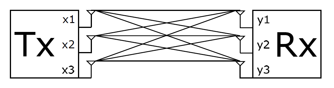
Bandwitdh in wireless communications is expensive and limited due to licensing. An easy way to use available bandwidth as efficient as possible is to add antennas on both the sending and transmitting side. This way a simple point to point transmission channel becomes a Multiple-Output-Multiple-Input (MIMO) system. A MIMO system without noise can be described by $$ \begin{pmatrix} y_1 \\ y_2 \\ \vdots \\ y_N \end{pmatrix} = \begin{pmatrix} h_{y_1 x_1} & h_{y_1 x_2} & \cdots & h_{y_1 x_M} \\ h_{y_2 x_1} & h_{y_2 x_2} & \cdots & h_{y_2 x_M} \\ \vdots & \vdots & \ddots & \vdots \\ h_{y_N x_1} & h_{y_N x_2} & \cdots & h_{y_N x_M} \\ \end{pmatrix} \begin{pmatrix} x_1 \\ x_2 \\ \vdots \\ x_M \end{pmatrix} $$ where

• $x_1, x_2, ..., x_M$ denote the sent data streams
• $y_1, y_2, ..., y_N$ denote the received data streams
• $N$ is the number of receiver antennas
• $M$ is the number of transmitter antennas
• $h_{xy}$ denotes the elements of the impulse response matrix $\mathbf{H}$

The spatial distribution of the antennas adds another dimension to the transmission link. By utilizing spatial multiplexing and sending independent data streams also called spatial streams theoretically a data rate increased by the factor $\min(M,N)$ is possible. These additional channels although are not completely independent from each other because signals are transmitted in the same time and frequency domain which leads to correlation. If the individual channels are correlated too much the receiver cannot distinguish between the sent spatial streams and therefore the channel capacity decreases. In conventional Single-Input-Single-Output (SISO) systems, multipath propagation and the random fading caused by it pose an obstacle. In MIMO systems this phenomenon can be exploited because the random fading provides an environment where the individual channels are highly decorrelated [4, 8, 9, 10]. The picture below shows an $3\times3$ MIMO system.

The 802.11n mimo model is a Kronecker correlation model which utilizes correlation matrices to describe the MIMO system. Using this method only parameters like angular spread, angle of incidence (arrival/departure) are needed. Contrary to ray tracing an exact description of the environment is not necessary. The channel impulse response matrix $\mathbf{H}$ for each path at a given time is described by $$ \mathbf{H} = \sqrt{P}\left(\sqrt{\frac{K}{K+1}} \begin{bmatrix} \mathrm{e}^{j\phi_{11}} & \mathrm{e}^{j\phi_{12}} & \mathrm{e}^{j\phi_{13}} \\ \mathrm{e}^{j\phi_{21}} & \mathrm{e}^{j\phi_{22}} & \mathrm{e}^{j\phi_{23}} \\ \mathrm{e}^{j\phi_{31}} & \mathrm{e}^{j\phi_{32}} & \mathrm{e}^{j\phi_{33}} \\ \end{bmatrix} + \sqrt{\frac{1}{K+1}} \begin{bmatrix} X_{11} & X_{12} & X_{13} \\ X_{21} & X_{22} & X_{23} \\ X_{31} & X_{32} & X_{33} \\ \end{bmatrix}\right) $$ where

• $X_{ij}$ are correlated, zero-mean, unit variance, complex Gaussian random variables
• $\exp{(j\phi_{ij})}$ are the elements of the fixed LOS matrix
• $K$ denotes the Ricean K-factor
• $P$ denotes the power of each tap

The 802.11n channel model utilizes cross correlation functions presented in [11] to derive the transmit and receive correlation matrices. The correlated zero-mean, unit variance, complex Gaussian random variables are then derived by $$ [X]=([R_{\mathrm{TX}}] \otimes [R_{\mathrm{RX}}])^{1/2}[\mathbf{H_{\mathrm{iid}}}] $$ where

• $R_{\mathrm{TX}}$ denotes the transmit correlation matrix
• $R_{\mathrm{RX}}$ denotes the receive correlation matrix
• $\mathbf{H_{\mathrm{iid}}}$ is a matrix of independent, zero-mean, unit variance, complex Gaussian random variables
• $\otimes$ denotes the Kronecker product operator (an example of an Kronecker product is provided below)

$$ \mathbf{C} = \mathbf{A} \otimes \mathbf{B} = \begin{pmatrix} a_{11}\mathbf{B} & \cdots & a_{1n}\mathbf{B} \\ \vdots & \ddots & \vdots \\ a_{m1}\mathbf{B} & \cdots & a_{mn}\mathbf{B} \\ \end{pmatrix} $$ where

• $\mathbf{A}$ denotes an $m \times n$ matrix
• $\mathbf{B}$ denotes an $x \times y$ matrix