Angle estimation

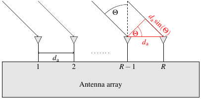
The angle can be determined with the induced phase differences between the antennas of an antenna array. The distance between the antennas is known and usually designed to be $d_\mathrm{a}=\frac{\lambda}{2}=\frac{c_0}{2f_\mathrm{C}}$. Due to $d_\mathrm{a}$, a signal at an angle $\Theta$ has to travel a distance $d_a\sin(\Theta)$ between antennas. This leads to a phase difference $e^{j\Omega_{\Theta}}$ of the received signals between each antenna. Under the assumption of a planar wavefront of reflections, which can be regarded as fulfilled after a distance of a few centimetres, the angle of arrival $\Theta$ can be trigonometrically determined with the phase difference [8].

By estimating the complex sinusoid frequency \begin{equation} \label{eqn:AngleFrequency} \Omega_{\Theta}=\frac{2\pi f_\mathrm{C}d_\mathrm{a}\sin(\Theta)}{c_0}, \end{equation} the angle of arrival $\Theta$ can be determined by, \begin{equation} \label{eqn:Angle} \Theta=\arcsin\left(\frac{\hat{\Omega}_{\Theta}c_0}{2\pi d_\mathrm{a}}\right). \end{equation}

$\Theta$ is only unambiguous for \begin{equation} \left|\frac{2\pi f_\mathrm{C}d_\mathrm{a}\sin(\Theta)}{c_0}\right|<\pi, \end{equation} which leads to: \begin{equation} \label{eqn:AngleUnambiguous} \Theta_{unamb}=\pm\arcsin\left(\frac{\lambda}{2d_\mathrm{a}}\right). \end{equation} By choosing $d_\mathrm{a}=\frac{\lambda}{2}$ the unambiguous range is maximzed to $\pm\pi/2$ or $\pm90^{\circ}$. This means that only objects at a maximum angle of $\Theta_\mathrm{unamb,max}=\pm90^{\circ}$ can be correctly identified.

The angle resolution is not linear and deteriorates towards higher angles. The angle resolution $\Delta \Theta$ at an angle of arrival $\Theta$ is inversely proportional to the number of antennas $R$, the space between antennas $d_\mathrm{a}$ and $\Theta$, \begin{equation} \Delta \Theta=\frac{c_0}{Rd_\mathrm{a}\cos{\Theta}f_\mathrm{C}}. \end{equation}

Distance angle periodogram

The periodogram can be applied in similar fashion as in the distance velocity periodogram. Angle estimation requires more than one receive antenna since the phase shift between antennas needs to be determined. The input matrix $(\mathbf{F})_{k,r}$ therefore needs to contain the same OFDM symbol from each antenna \begin{equation} \label{eqn:AngleInputMatrix} (\mathbf{F})_{k,r}= \begin{bmatrix} c_{0,0}&\cdots&c_{0,R-1}\\\vdots&\ddots&\vdots\\ c_{N-1,0}&\cdots&c_{N-1,R-1}\\ \end{bmatrix}, \in \mathbb{C}^{N\times R}. \end{equation}

The estimation of $\hat{\Omega}_d$ and $\hat{\Omega}_{\Theta}$ is analog to the distance velocity periodogram. \begin{align} Per_{s(k)}(n,r)&=\frac{1}{NR}\left|\sum_{k=0}^{N_\mathrm{Per}-1}{\left(\sum_{l=0}^{R_\mathrm{Per}-1}{(\mathbf{F})_{k,r}e^{-j2\pi \frac{lr}{R_\mathrm{Per}}}}\right)e^{j2\pi \frac{nk}{N_\mathrm{Per}}}}\right|^2 \nonumber \\ &=\frac{1}{NR}\left|CPer_{\mathbf F}(n,r)\right|^2. \end{align} The resulting matrix of $Per_{s(k)}(f)$ is of shape $N_\mathrm{Per}\times R_\mathrm{Per}$. The corresponding sinusoid frequencies of the rows and columns are determined by $\hat{\Omega}_\mathrm{d}=2 \pi \hat{n}/N_\mathrm{Per}$ and $\hat{\Omega}_{\Theta}=\pi \hat{r}/R_\mathrm{Per}$. The peaks can be translated to targets at: \begin{align} \hat{d}&=\frac{\hat{n}c_0}{2\Delta f N_\mathrm{Per}},\\ \hat{\Theta}&=\arcsin\left(\frac{\hat{r}c_0}{\pi d_\mathrm{a}R_\mathrm{Per}}\right). \end{align}