Where $m_S=W-1$, which equals the number of memory elements of the convolutional-encoder.
The submatrices $\mathbf{H_{\mathit{i}}}$ are defined by the underlying block code with dimensions ${b\times c}$ and can be arbitrary. However, a powerful block code such as the regular $\left(d_{v}=3,d_{c}=6\right)$ LDPC code increases the performance of the SC-LDPC code. Additionally, the submatrices can be time-varying $\mathbf{H_{\mathit{i}}}(t)$, which leads to $$ \mathbf{H}_{conv,\infty}\left(t\right)=\left(\begin{array}{ccccc} \ddots\\ \ddots & \mathbf{H}_{0}\left(t\right)\\ \ddots & \mathbf{H}_{1}\left(t\right) & \mathbf{H}_{0}\left(t+1\right)\\ \ddots & \vdots & \mathbf{H}_{1}\left(t+1\right) & \mathbf{H}_{0}\left(t+2\right)\\ & \mathbf{H}_{m_{S}}\left(t\right) & \vdots & \mathbf{H}_{1}\left(t+2\right) & \ddots\\ & & \mathbf{H}_{m_{S}}\left(t+1\right) & \vdots & \ddots\\ & & & \mathbf{H}_{m_{S}}\left(t+2\right) & \ddots\\ & & & & \ddots \end{array}\right)_{\infty}. $$
This webdemo uses random submatrices, hence the sub matrices can be seen as time-varying. The code rate for infinite SC-LDPC codes ${R_{C,\infty}}$, is equal to the code rate of the underlying block code and thus $$ R_{C,\infty}=1-\frac{b}{c}. $$
On the other hand, practical systems need a termination after a couple of replications ${L}$, this structure can be represented by a finite matrix $$ \mathbf{H}_{conv}=\left(\begin{array}{ccccc} \mathbf{H}_{0}\\ \mathbf{H}_{1} & \mathbf{H}_{0}\\ \vdots & \mathbf{H}_{1} & \ddots\\ \mathbf{H_{\mathit{m_{S}}}} & \vdots & \ddots & \mathbf{H}_{0}\\ & \mathbf{H_{\mathrm{m_{S}}}} & \ddots & \mathbf{H}_{1} & \mathbf{H}_{0}\\ & & & \vdots & \mathbf{H}_{1}\\ & & & \mathbf{H}_{\mathrm{m_{S}}} & \vdots\\ & & & & \mathbf{H}_{m_{S}} \end{array}\right)_{(L+m_{S})\,\times\,L}. $$
The terminated SC-LDPC code is still a block code with a very large block length. However, the properties of the spatial coupling dominate the code behavior, even though the standard belief propagation (BP) decoder can still be used. An optimized windowed decoder exists to reduce the decoding complexity and the number of decoding iterations for these very large codes.
The design code rate of a terminated SC-LDPC code can be approximated by $$ R_D=1-\frac{L+m_S}{L}\cdot\frac{d_v}{d_c}. $$
Tail-biting SC-LDPC Codes
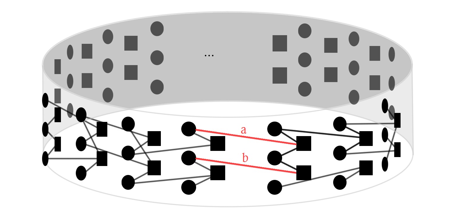
Tail-biting SC-LDPC codes describes one way to mitigate the rate loss of a terminated SC-LDPC code. Instead of a termination, the last $m_{S}$ blocks are connected with the first ${m_{S}}$ blocks of a SC-LDPC code.
In comparison to the terminated SC-LDPC code, the tail-biting code has a constant code rate, since the code structure looks like a ring structure without termination and therefore no rate loss occurs.
In matrix representation tail-biting connects the “tail” with the “head” by use of an upper triangle structure of the matrix.
However, the effect of threshold saturation (good decoding performance under BP decoding) does not occur and the performance is similar to the BP-performance of the underlying block LDPC code.
For finite length codes the performance increases because the code length increases, which is known as finite length effect. Comparing $\mathbf{\mathbf{H}_{\mathrm{\mathit{\mathrm{conv,tail}}}}}$ and a random block LDPC matrix
$\mathbf{\mathbf{H}_{\mathrm{rand}}}$ with same dimensions, leads to the same results.
For $\mathit{m{}_{S}=2}$, the check matrix $\mathbf{\mathbf{H}_{\mathrm{conv}}}$ of a tail-biting SC-LDPC is
$$
\mathbf{H}_{\mathrm{conv,tail}}=\left(\begin{array}{ccccccc}
\mathbf{H_{\mathit{2}}} & \mathbf{H_{\mathit{1}}} & \mathbf{H_{\mathit{0}}}\\
& \mathbf{H_{\mathit{2}}} & \mathbf{H_{\mathit{1}}} & \mathbf{H_{\mathit{0}}}\\
& & \mathbf{H_{\mathit{2}}} & \mathbf{H_{\mathit{1}}} & \mathbf{H_{\mathit{0}}}\\
\vdots & \vdots & & \ddots & \ddots & \ddots\\
& & & & \mathbf{H_{\mathit{2}}} & \mathbf{H_{\mathit{1}}} & \mathbf{H_{\mathit{0}}}\\
{\mathbf{H_{\mathit{0}}}} & & & & & \mathbf{H_{\mathit{2}}} & \mathbf{H_{\mathit{1}}}\\
{\mathbf{H}_{\mathit{1}}} & {\mathbf{H_{\mathit{0}}}} & & & & & \mathbf{H_{\mathit{2}}}
\end{array}\right)_{L\,\times\,L}.
$$
Thus, the design code rate of a tail-biting SC-LDPC code is
$$
R_D=1-\frac{d_v}{d_c}.
$$
